Loading
Loading
Loading

Download pamphlet

Anthrobotanica Investigations

Plant Bio-signal Data Exploration & Feature Classification


Intro

This is an exploration of the bio-signals produced by a baby rubberplant (Peperomia obtusifolia). The houseplant has a robotic prosthesis that moves based on the plant's bio-signals. Four surface electrodes are each attached to a leaf, the signals are amplified 100x and fed to a script that controls the prosthesis motors.

In [1]:
from glob import glob
from os import listdir
from os.path import join
import numpy as np
import pandas as pd
import matplotlib.pyplot as plt
import matplotlib.patches as mpatches
import random
from scipy import stats

# Enable interactive matplotlib plots
%matplotlib notebook

Data Acquisition

The baby rubberplant has surface electrodes on four of its leaves which are connected to the prosthesis computer by insulated coaxial cables.

Sensor data is collected as comma separated files (.csv) in the folder /datasets grouped by stimuli and electrode channel (i.e. the leaf that is stimulated). Each dataset are approximately 10 minutes recording of 4 single-ended channels at 140 Hz in 16-bit resolution. Each channel is amplified 100x by LM358 op-amps and read by ADS1115 16-bit analog-to-digital converter.

Under is the code used for data gathering. The whole script, ads1115-to-csv.py, is in the current folder.

f = open("log.csv", "w", newline="")
c = csv.writer(f)

c.writerow(["Datetime", "chan0", "chan1", "chan2", "chan3"]) # List of fieldnames
for i in range(SAMPLES):
    c.writerow([datetime.now().isoformat(sep=' ', timespec='milliseconds'), 
                "{:8.6f}".format(chan0.voltage),
                "{:8.6f}".format(chan1.voltage), 
                "{:8.6f}".format(chan2.voltage), 
                "{:8.6f}".format(chan3.voltage)])

f.close()

The biosignals are grouped in the following folders:

/datasets/baseline
No light source, approximately 1 week since watering.

../chan_0_light, chan_1_light, chan_2_light, chan_3_light
The denoted channel has a lightbulb with artificial sunlight approx. 10 centimeter from the leaf, while the three other channels are covered with a dark blanket.

../drought
Approx. 10 minutes recording with dry soil (1 month since watering) plus soaked soil.

../chan_0_pain, chan_1_pain, chan_2_pain, chan_3_pain
The leaf corresponding to the channel has been cut after approx. 10 minutes baseline recording. The cut is 5 millimeter long from the outside of the leaf blade in proximity to the surface sensor.

In [2]:
# Import datasets and set 'Datetime' column as dataset index
datasets = glob('datasets/*.csv')
dfs = {}

for filename in datasets:
    df = pd.read_csv(filename)
    df['Datetime'] = pd.to_datetime(df['Datetime'], format='%Y-%m-%d %H:%M:%S.%f')
    df = df.set_index('Datetime')
    dfs[str(filename)[9:-4]] = df

Data Analysis

In [3]:
dfs['baseline'].describe()
Out[3]:
chan0 chan1 chan2 chan3
count 250000.000000 250000.000000 250000.000000 250000.000000
mean 1.599891 1.742485 1.670655 1.678602
std 0.001305 0.002980 0.002638 0.000485
min 1.593049 1.734053 1.662426 1.671801
25% 1.598799 1.739803 1.668551 1.678301
50% 1.599924 1.742553 1.670676 1.678551
75% 1.600924 1.745178 1.672676 1.678926
max 1.605549 1.749303 1.679176 1.682801

Previews of the different sensor data:

In [4]:
alpha_val = 0.7 # Signal smoothing by exponential moving averages. Small weighting factor results in high degree of smoothing, larger value provides quicker response to recent changes.
fig, axes = plt.subplots(nrows=3, ncols=4, figsize=(8,5))
dfs['baseline'].ewm(alpha=alpha_val).mean().plot(ax=axes[0,0], legend=None, xlabel=None).tick_params(top=False, bottom=False, left=False, right=False, labelleft=False, labelbottom=False)
axes[0,0].set_title("Baseline")
axes[0,0].set_xlabel('')
dfs['drought'].ewm(alpha=alpha_val).mean().plot(ax=axes[0,1], legend=None).tick_params(top=False, bottom=False, left=False, right=False, labelleft=False, labelbottom=False)
axes[0,1].set_title("Drought")
axes[0,1].set_xlabel('')
axes[0,2].set_visible(False)
axes[0,3].set_visible(False)
dfs['chan_0_light'].ewm(alpha=alpha_val).mean().plot(ax=axes[1,0], legend=None).tick_params(top=False, bottom=False, left=False, right=False, labelleft=False, labelbottom=False)
axes[1,0].set_title("Chn 0 light")
axes[1,0].set_xlabel('')
axes[1,0].set_ylabel('Signal Voltage')
dfs['chan_1_light'].ewm(alpha=alpha_val).mean().plot(ax=axes[1,1], legend=None).tick_params(top=False, bottom=False, left=False, right=False, labelleft=False, labelbottom=False)
axes[1,1].set_title("Chn 1 light")
axes[1,1].set_xlabel('')
dfs['chan_2_light'].ewm(alpha=alpha_val).mean().plot(ax=axes[1,2], legend=None).tick_params(top=False, bottom=False, left=False, right=False, labelleft=False, labelbottom=False)
axes[1,2].set_title("Chn 2 light")
axes[1,2].set_xlabel('')
dfs['chan_3_light'].ewm(alpha=alpha_val).mean().plot(ax=axes[1,3], legend=None).tick_params(top=False, bottom=False, left=False, right=False, labelleft=False, labelbottom=False)
axes[1,3].set_title("Chn 3 light")
axes[1,3].set_xlabel('')
dfs['chan_0_pain'].ewm(alpha=alpha_val).mean().plot(ax=axes[2,0], legend=None).tick_params(top=False, bottom=False, left=False, right=False, labelleft=False, labelbottom=False)
axes[2,0].set_title("Chn 0 pain")
axes[2,0].set_xlabel('')
dfs['chan_1_pain'].ewm(alpha=alpha_val).mean().plot(ax=axes[2,1], legend=None).tick_params(top=False, bottom=False, left=False, right=False, labelleft=False, labelbottom=False)
axes[2,1].set_title("Chn 1 pain")
axes[2,1].set_xlabel('Time Axis')
axes[2,1].xaxis.set_label_coords(1.05, -0.05)
dfs['chan_2_pain'].ewm(alpha=alpha_val).mean().plot(ax=axes[2,2], legend=None).tick_params(top=False, bottom=False, left=False, right=False, labelleft=False, labelbottom=False)
axes[2,2].set_title("Chn 2 pain")
axes[2,2].set_xlabel('')
dfs['chan_3_pain'].ewm(alpha=alpha_val).mean().plot(ax=axes[2,3], legend=None).tick_params(top=False, bottom=False, left=False, right=False, labelleft=False, labelbottom=False)
axes[2,3].set_title("Chn 3 pain")
axes[2,3].set_xlabel('')
plt.tight_layout()
plt.show()
"); if (!fig.cell_info) { console.error('Failed to find cell for figure', id, fig); return; } fig.cell_info[0].output_area.element.one( 'cleared', { fig: fig }, fig._remove_fig_handler ); }; mpl.figure.prototype.handle_close = function (fig, msg) { var width = fig.canvas.width / fig.ratio; fig.cell_info[0].output_area.element.off( 'cleared', fig._remove_fig_handler ); // Update the output cell to use the data from the current canvas. fig.push_to_output(); var dataURL = fig.canvas.toDataURL(); // Re-enable the keyboard manager in IPython - without this line, in FF, // the notebook keyboard shortcuts fail. IPython.keyboard_manager.enable(); fig.parent_element.innerHTML = ''; fig.close_ws(fig, msg); }; mpl.figure.prototype.close_ws = function (fig, msg) { fig.send_message('closing', msg); // fig.ws.close() }; mpl.figure.prototype.push_to_output = function (_remove_interactive) { // Turn the data on the canvas into data in the output cell. var width = this.canvas.width / this.ratio; var dataURL = this.canvas.toDataURL(); this.cell_info[1]['text/html'] = ''; }; mpl.figure.prototype.updated_canvas_event = function () { // Tell IPython that the notebook contents must change. IPython.notebook.set_dirty(true); this.send_message('ack', {}); var fig = this; // Wait a second, then push the new image to the DOM so // that it is saved nicely (might be nice to debounce this). setTimeout(function () { fig.push_to_output(); }, 1000); }; mpl.figure.prototype._init_toolbar = function () { var fig = this; var toolbar = document.createElement('div'); toolbar.classList = 'btn-toolbar'; this.root.appendChild(toolbar); function on_click_closure(name) { return function (_event) { return fig.toolbar_button_onclick(name); }; } function on_mouseover_closure(tooltip) { return function (event) { if (!event.currentTarget.disabled) { return fig.toolbar_button_onmouseover(tooltip); } }; } fig.buttons = {}; var buttonGroup = document.createElement('div'); buttonGroup.classList = 'btn-group'; var button; for (var toolbar_ind in mpl.toolbar_items) { var name = mpl.toolbar_items[toolbar_ind][0]; var tooltip = mpl.toolbar_items[toolbar_ind][1]; var image = mpl.toolbar_items[toolbar_ind][2]; var method_name = mpl.toolbar_items[toolbar_ind][3]; if (!name) { /* Instead of a spacer, we start a new button group. */ if (buttonGroup.hasChildNodes()) { toolbar.appendChild(buttonGroup); } buttonGroup = document.createElement('div'); buttonGroup.classList = 'btn-group'; continue; } button = fig.buttons[name] = document.createElement('button'); button.classList = 'btn btn-default'; button.href = '#'; button.title = name; button.innerHTML = ''; button.addEventListener('click', on_click_closure(method_name)); button.addEventListener('mouseover', on_mouseover_closure(tooltip)); buttonGroup.appendChild(button); } if (buttonGroup.hasChildNodes()) { toolbar.appendChild(buttonGroup); } // Add the status bar. var status_bar = document.createElement('span'); status_bar.classList = 'mpl-message pull-right'; toolbar.appendChild(status_bar); this.message = status_bar; // Add the close button to the window. var buttongrp = document.createElement('div'); buttongrp.classList = 'btn-group inline pull-right'; button = document.createElement('button'); button.classList = 'btn btn-mini btn-primary'; button.href = '#'; button.title = 'Stop Interaction'; button.innerHTML = ''; button.addEventListener('click', function (_evt) { fig.handle_close(fig, {}); }); button.addEventListener( 'mouseover', on_mouseover_closure('Stop Interaction') ); buttongrp.appendChild(button); var titlebar = this.root.querySelector('.ui-dialog-titlebar'); titlebar.insertBefore(buttongrp, titlebar.firstChild); }; mpl.figure.prototype._remove_fig_handler = function (event) { var fig = event.data.fig; fig.close_ws(fig, {}); }; mpl.figure.prototype._root_extra_style = function (el) { el.style.boxSizing = 'content-box'; // override notebook setting of border-box. }; mpl.figure.prototype._canvas_extra_style = function (el) { // this is important to make the div 'focusable el.setAttribute('tabindex', 0); // reach out to IPython and tell the keyboard manager to turn it's self // off when our div gets focus // location in version 3 if (IPython.notebook.keyboard_manager) { IPython.notebook.keyboard_manager.register_events(el); } else { // location in version 2 IPython.keyboard_manager.register_events(el); } }; mpl.figure.prototype._key_event_extra = function (event, _name) { var manager = IPython.notebook.keyboard_manager; if (!manager) { manager = IPython.keyboard_manager; } // Check for shift+enter if (event.shiftKey && event.which === 13) { this.canvas_div.blur(); // select the cell after this one var index = IPython.notebook.find_cell_index(this.cell_info[0]); IPython.notebook.select(index + 1); } }; mpl.figure.prototype.handle_save = function (fig, _msg) { fig.ondownload(fig, null); }; mpl.find_output_cell = function (html_output) { // Return the cell and output element which can be found *uniquely* in the notebook. // Note - this is a bit hacky, but it is done because the "notebook_saving.Notebook" // IPython event is triggered only after the cells have been serialised, which for // our purposes (turning an active figure into a static one), is too late. var cells = IPython.notebook.get_cells(); var ncells = cells.length; for (var i = 0; i < ncells; i++) { var cell = cells[i]; if (cell.cell_type === 'code') { for (var j = 0; j < cell.output_area.outputs.length; j++) { var data = cell.output_area.outputs[j]; if (data.data) { // IPython >= 3 moved mimebundle to data attribute of output data = data.data; } if (data['text/html'] === html_output) { return [cell, data, j]; } } } } }; // Register the function which deals with the matplotlib target/channel. // The kernel may be null if the page has been refreshed. if (IPython.notebook.kernel !== null) { IPython.notebook.kernel.comm_manager.register_target( 'matplotlib', mpl.mpl_figure_comm ); }

Daniel Slåttnes [Norway]
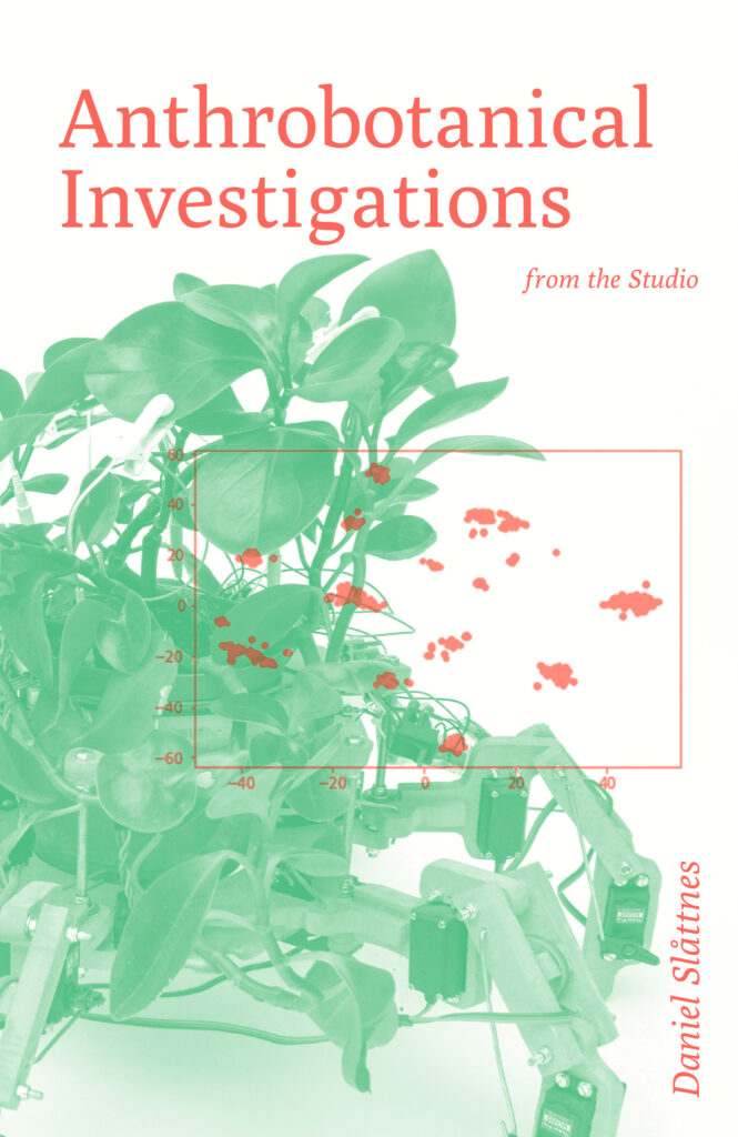
Plant Cyborgs, from the series Anthrobotanical Investigations, 2015-ongoing.
Peperomia obtusifolia (baby rubber plant), electronic and robotic components, software for tracing the plant’s biosignals and moving robotic prostheses.

“The plant is like an individual with whom I am trying to establish a relationship. What does it want? We cannot understand each other, we will never be able to share everything. But we can share our time together, our mutual relationship.” –Daniel Slåttnes, Anthrobotanical Investigations from the Studio

Daniel Slåttnes Plant Cyborgs are an ongoing interspecies collaboration. Although one might assume at first glance that these plant-machine hybrids are a byproduct of the technoscientific pursuit of control, Slåttnes applies his considerable engineering and programming skills to listen to plants, to sculpt with them, and perhaps eventually, to dance with them. To create the series of works from which the cyborgs originated, he began by meditating with the plant, sometimes for hours at a time.He then developed ways to record and amplify his own biosignals and the plant’s, mediating energy and movement into a kind of soundtrack that both parties produce in relation to one another. 

Daniel Slåttnes lives and works in Oslo, Norway, and Västra Ämtervik, Sweden. Consciousness in plants, investigations into objecthood, and the shape of time are examples of topics he has been researching in recent years. He explores in several of his works possibilities to establish a kind of communication with the materials he works with. The meeting between plant and machine is a distinct focus as they are both on the outskirts of what we perceive as conscious life.

Links

Pioneering botanical bioartist George Gessert responds to Plant Cyborgs here.